45 data labels excel pie chart
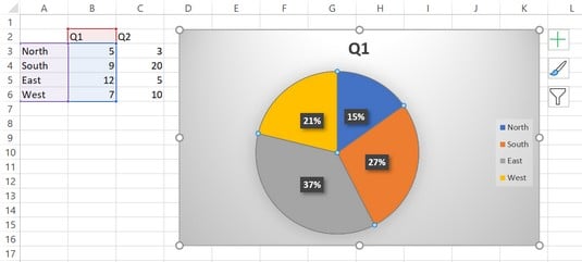
Pie Chart in Excel | How to Create Pie Chart - EDUCBA Pie Chart in Excel is used for showing the completion or main contribution of different segments out of 100%. It is like each value represents the portion of the Slice from the total complete Pie. For Example, we have 4 values A, B, C and D. › excel-pie-chartExcel Pie Chart - How to Create & Customize? (Top 5 Types) #Adding Data Labels. We will customize the Pie Chart in Excel by Adding Data Labels. Scenario 1: The procedure to add data labels are as follows: Click on the Pie Chart > click the ‘+’ icon > check/tick the “Data Labels” checkbox in the “Chart Element” box > select the “Data Labels” right arrow > select the “Outside End” option.
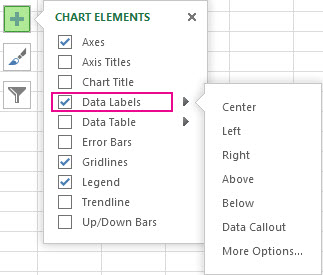
Add or remove data labels in a chart - support.microsoft.com Click the data series or chart. To label one data point, after clicking the series, click that data point. In the upper right corner, next to the chart, click Add Chart Element > Data Labels. To change the location, click the arrow, and choose an option. If you want to show your data label inside a text bubble shape, click Data Callout.

Data labels excel pie chart
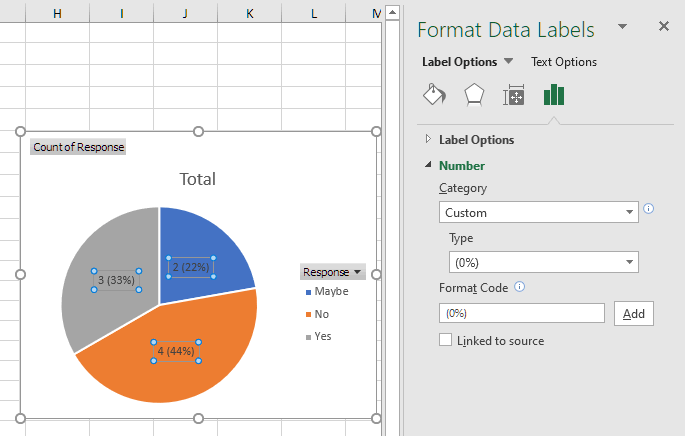
› pie-chart-excelHow to Create a Pie Chart in Excel | Smartsheet Aug 27, 2018 · To create a pie chart in Excel 2016, add your data set to a worksheet and highlight it. Then click the Insert tab, and click the dropdown menu next to the image of a pie chart. Select the chart type you want to use and the chosen chart will appear on the worksheet with the data you selected. How To Change Data Labels In Excel Pie Chart - JawabSoal.ID Ada banyak pertanyaan tentang how to change data labels in excel pie chart beserta jawabannya di sini atau Kamu bisa mencari soal/pertanyaan lain yang berkaitan dengan how to change data labels in excel pie chart menggunakan kolom pencarian di bawah ini. excel - How to not display labels in pie chart that are 0% - Stack Overflow Generate a new column with the following formula: =IF (B2=0,"",A2) Then right click on the labels and choose "Format Data Labels". Check "Value From Cells", choosing the column with the formula and percentage of the Label Options. Under Label Options -> Number -> Category, choose "Custom". Under Format Code, enter the following:
Data labels excel pie chart. How to Create and Format a Pie Chart in Excel - Lifewire Select the plot area of the pie chart. Select a slice of the pie chart to surround the slice with small blue highlight dots. Drag the slice away from the pie chart to explode it. To reposition a data label, select the data label to select all data labels. Select the data label you want to move and drag it to the desired location. How to Make a Pie Chart with Multiple Data in Excel (2 Ways) - ExcelDemy In Pie Chart, we can also format the Data Labels with some easy steps. These are given below. Steps: First, to add Data Labels, click on the Plus sign as marked in the following picture. After that, check the box of Data Labels. At this stage, you will be able to see that all of your data has labels now. Change the format of data labels in a chart To get there, after adding your data labels, select the data label to format, and then click Chart Elements > Data Labels > More Options. To go to the appropriate area, click one of the four icons ( Fill & Line, Effects, Size & Properties ( Layout & Properties in Outlook or Word), or Label Options) shown here. Data Labels in Excel Pivot Chart (Detailed Analysis) 7 Suitable Examples with Data Labels in Excel Pivot Chart Considering All Factors 1. Adding Data Labels in Pivot Chart 2. Set Cell Values as Data Labels 3. Showing Percentages as Data Labels 4. Changing Appearance of Pivot Chart Labels 5. Changing Background of Data Labels 6. Dynamic Pivot Chart Data Labels with Slicers 7.
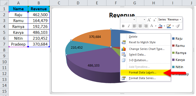
How to display leader lines in pie chart in Excel? - ExtendOffice To display leader lines in pie chart, you just need to check an option then drag the labels out. 1. Click at the chart, and right click to select Format Data Labels from context menu. 2. In the popping Format Data Labels dialog/pane, check Show Leader Lines in the Label Options section. See screenshot: trumpexcel.com › pie-chartHow to Make a PIE Chart in Excel (Easy Step-by-Step Guide) Creating a Pie Chart in Excel. To create a Pie chart in Excel, you need to have your data structured as shown below. The description of the pie slices should be in the left column and the data for each slice should be in the right column. Once you have the data in place, below are the steps to create a Pie chart in Excel: Select the entire dataset Pie Charts in Excel - How to Make with Step by Step Examples Thus, data labels make it easy to read and interpret an excel pie chart. Note: Data labels are directly linked to the data points of the source dataset. Therefore, the data labels automatically update with a change in the data points. Step 5: Right-click the pie chart again. Click the arrow of “add data labels” and select “add data ... How to Edit Pie Chart in Excel (All Possible Modifications) How to Edit Pie Chart in Excel 1. Change Chart Color 2. Change Background Color 3. Change Font of Pie Chart 4. Change Chart Border 5. Resize Pie Chart 6. Change Chart Title Position 7. Change Data Labels Position 8. Show Percentage on Data Labels 9. Change Pie Chart's Legend Position 10. Edit Pie Chart Using Switch Row/Column Button 11.
Move data labels - support.microsoft.com Right-click the selection > Chart Elements > Data Labels arrow, and select the placement option you want. Different options are available for different chart types. For example, you can place data labels outside of the data points in a pie chart but not in a column chart. How to Create a Pie Chart in Excel | Smartsheet Aug 27, 2018 · A pie chart, sometimes called a circle chart, is a useful tool for displaying basic statistical data in the shape of a circle (each section resembles a slice of pie).Unlike in bar charts or line graphs, you can only display a single data series in a pie chart, and you can’t use zero or negative values when creating one.A negative value will display as its positive equivalent, and … How to Make a Pie Chart in Excel & Add Rich Data Labels to The Chart! Creating and formatting the Pie Chart 1) Select the data. 2) Go to Insert> Charts> click on the drop-down arrow next to Pie Chart and under 2-D Pie, select the Pie Chart, shown below. 3) Chang the chart title to Breakdown of Errors Made During the Match, by clicking on it and typing the new title. Add or remove data labels in a chart - support.microsoft.com Data labels make a chart easier to understand because they show details about a data series or its individual data points. For example, in the pie chart below, without the data labels it would be difficult to tell that coffee was 38% of total sales. Depending on what you want to highlight on a chart, you can add labels to one series, all the ...
Add or remove data labels in a chart
How to Create a Graph in Excel: 12 Steps (with Pictures ... - wikiHow May 31, 2022 · Double-click the "Chart Title" text at the top of the chart, then delete the "Chart Title" text, replace it with your own, and click a blank space on the graph. On a Mac, you'll instead click the Design tab, click Add Chart Element , select Chart Title , …
/cookie-shop-revenue-58d93eb65f9b584683981556.jpg)
How to Create and Format a Pie Chart in Excel
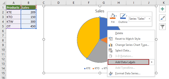
› make-pie-chart-in-excelPie Charts in Excel - How to Make with Step by Step Examples These percentages will appear as data labels on the pie chart. For adding such data labels, right-click the pie chart and choose “add data labels” from the context menu. • Method 2–Enter numbers as is in the series and let Excel convert them to percentages. Once converted, the numbers and percentages will appear as data labels on the ...

How to: Display and Format Data Labels | .NET File Format ...
Pie Chart in Excel – Inserting, Formatting, Filters, Data Labels Dec 29, 2021 · The total of percentages of the data point in the pie chart would be 100% in all cases. Consequently, we can add Data Labels on the pie chart to show the numerical values of the data points. We can use Pie Charts to represent: ratio of population of male and female of a country. proportion of online/offline payment modes of a local car rental ...
Pie Chart in Excel | How to Create Pie Chart | Step-by-Step ...
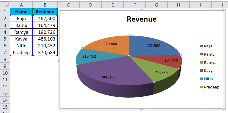
How to Make a PIE Chart in Excel (Easy Step-by-Step Guide) Creating a Pie Chart in Excel. To create a Pie chart in Excel, you need to have your data structured as shown below. The description of the pie slices should be in the left column and the data for each slice should be in the right column. Once you have the data in place, below are the steps to create a Pie chart in Excel: Select the entire dataset
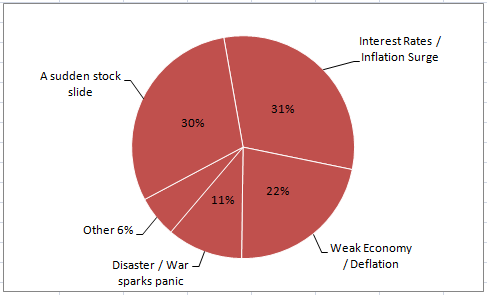
How to show percentage in pie chart in Excel?
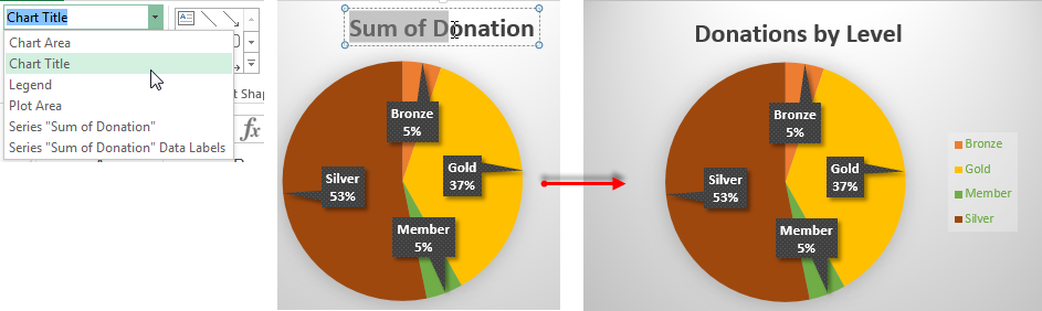
Edit titles or data labels in a chart - support.microsoft.com On a chart, click one time or two times on the data label that you want to link to a corresponding worksheet cell. The first click selects the data labels for the whole data series, and the second click selects the individual data label. Right-click the data label, and then click Format Data Label or Format Data Labels.
Create a Pie Chart in Excel (In Easy Steps)
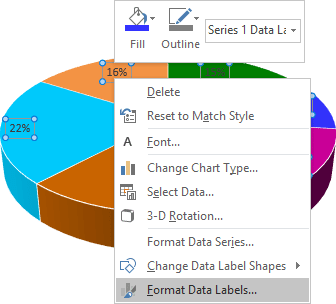
How to hide zero data labels in chart in Excel? - ExtendOffice If you want to hide zero data labels in chart, please do as follow: 1. Right click at one of the data labels, and select Format Data Labels from the context menu. See screenshot: 2. In the Format Data Labels dialog, Click Number in left pane, then select Custom from the Category list box, and type #"" into the Format Code text box, and click Add button to add it to Type list box.

How to insert data labels to a Pie chart in Excel 2013
Creating Pie Chart and Adding/Formatting Data Labels (Excel) Creating Pie Chart and Adding/Formatting Data Labels (Excel)

Change the format of data labels in a chart
› examples › pie-chartCreate a Pie Chart in Excel (In Easy Steps) - Excel Easy 6. Create the pie chart (repeat steps 2-3). 7. Click the legend at the bottom and press Delete. 8. Select the pie chart. 9. Click the + button on the right side of the chart and click the check box next to Data Labels. 10. Click the paintbrush icon on the right side of the chart and change the color scheme of the pie chart. Result: 11.
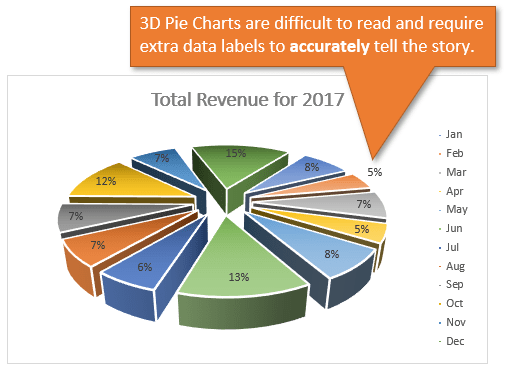
Excel 3-D Pie charts - Microsoft Excel 2016
excel - Pie Chart VBA DataLabel Formatting - Stack Overflow sub updatechartformat () with activeworkbook.sheets ("mhfa summary").chartobjects ("chart 4").activate with activechart.seriescollection (1).datalabels _ .showpercentage = true with activechart.seriescollection (1).datalabels _ .separator = "" & chr (10) & "" end with end with end with with activeworkbook.sheets ("mhfa …

How to data label on pie chart? - Simple Excel VBA
Change the format of data labels in a chart Excel for Microsoft 365 Word for Microsoft 365 Outlook for Microsoft 365 PowerPoint for Microsoft 365 Excel ... Data labels make a chart easier to understand because they show details about a data series or its individual data points. For example, in the pie chart below, without the data labels it would be difficult to tell that coffee was 38% ...
5 New Charts to Visually Display Data in Excel 2019 - dummies
Excel Pie Chart - How to Create & Customize? (Top 5 Types) #Adding Data Labels. We will customize the Pie Chart in Excel by Adding Data Labels. Scenario 1: The procedure to add data labels are as follows: Click on the Pie Chart > click the ‘+’ icon > check/tick the “Data Labels” checkbox in the “Chart Element” box > select the “Data Labels” right arrow > select the “Outside End” option.
Change the look of chart text and labels in Numbers on Mac ...
excelunlocked.com › pie-chart-in-excelPie Chart in Excel - Inserting, Formatting, Filters, Data Labels Dec 29, 2021 · The total of percentages of the data point in the pie chart would be 100% in all cases. Consequently, we can add Data Labels on the pie chart to show the numerical values of the data points. We can use Pie Charts to represent: ratio of population of male and female of a country. proportion of online/offline payment modes of a local car rental ...

Create a Dynamic Pie Chart with Dynamic Legend in Excel which ...
Create a Pie Chart in Excel (In Easy Steps) - Excel Easy 6. Create the pie chart (repeat steps 2-3). 7. Click the legend at the bottom and press Delete. 8. Select the pie chart. 9. Click the + button on the right side of the chart and click the check box next to Data Labels. 10. Click the paintbrush icon on the right side of the chart and change the color scheme of the pie chart. Result: 11.
Is there a way to prevent pie chart data labels from ...
› documents › excelHow to hide zero data labels in chart in Excel? - ExtendOffice If you want to hide zero data labels in chart, please do as follow: 1. Right click at one of the data labels, and select Format Data Labels from the context menu. See screenshot: 2. In the Format Data Labels dialog, Click Number in left pane, then select Custom from the Category list box, and type #"" into the Format Code text box, and click Add button to add it to Type list box.
Move data labels
How to make a pie chart in Excel with words - profitclaims.com Select the range A1:D1, hold down CTRL and select the range A3:D3. 6. Create the pie chart (repeat steps 2-3). 7. Click the legend at the bottom and press Delete. 8. Select the pie chart. 9. Click the + button on the right side of the chart and click the check box next to Data Labels.
KB209780: Data labels overlap when exporting a pie graph in a ...
How to add data labels from different column in an Excel chart? Right click the data series in the chart, and select Add Data Labels > Add Data Labels from the context menu to add data labels. 2. Click any data label to select all data labels, and then click the specified data label to select it only in the chart. 3.

Pie Chart – Excel Tutorial
excel - How to not display labels in pie chart that are 0% - Stack Overflow Generate a new column with the following formula: =IF (B2=0,"",A2) Then right click on the labels and choose "Format Data Labels". Check "Value From Cells", choosing the column with the formula and percentage of the Label Options. Under Label Options -> Number -> Category, choose "Custom". Under Format Code, enter the following:

Creating Pie Chart and Adding/Formatting Data Labels (Excel)
How To Change Data Labels In Excel Pie Chart - JawabSoal.ID Ada banyak pertanyaan tentang how to change data labels in excel pie chart beserta jawabannya di sini atau Kamu bisa mencari soal/pertanyaan lain yang berkaitan dengan how to change data labels in excel pie chart menggunakan kolom pencarian di bawah ini.
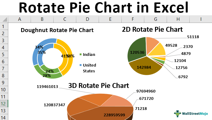
Rotate Pie Chart in Excel | How to Rotate Pie Chart in Excel?
› pie-chart-excelHow to Create a Pie Chart in Excel | Smartsheet Aug 27, 2018 · To create a pie chart in Excel 2016, add your data set to a worksheet and highlight it. Then click the Insert tab, and click the dropdown menu next to the image of a pie chart. Select the chart type you want to use and the chosen chart will appear on the worksheet with the data you selected.

How-to Add Label Leader Lines to an Excel Pie Chart - Excel ...
Create Outstanding Pie Charts in Excel | Pryor Learning

How to Make a Pie Chart in Excel & Add Rich Data Labels to ...

Excel VBA Codebase: Hide all data label less than any ...

Change color of data label placed, using the 'best fit ...

How to fix wrapped data labels in a pie chart | Sage Intelligence

How to Change Excel Chart Data Labels to Custom Values?
:max_bytes(150000):strip_icc()/Capture-5c84951cc9e77c0001f2ac82.JPG)
How to Create and Format a Pie Chart in Excel

Change the format of data labels in a chart
How to ☝️Make a Pie Chart in Excel (Free Template ...
How-to Make a WSJ Excel Pie Chart with Labels Both Inside and ...

How to make a pie chart in Excel

How to Data Labels in a Pie chart in Excel 2010

Creating Graphs in Excel 2013

How to Make a Pie Chart in Excel - All Things How
Excel custom pie chart labels - Microsoft Community

Office: Display Data Labels in a Pie Chart

How to Make Pie Chart with Labels both Inside and Outside ...

Custom data labels in a chart
When to use Pie Charts in Dashboards - Best Practices | Excel ...
KB209780: Data labels overlap when exporting a pie graph in a ...

How to Make an Excel Pie Chart

Change the format of data labels in a chart
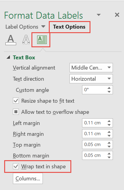
How to fix wrapped data labels in a pie chart | Sage Intelligence
Pie Chart in Excel | How to Create Pie Chart | Step-by-Step ...

How to Make Pie Chart with Labels both Inside and Outside ...
Post a Comment for "45 data labels excel pie chart"